There’s always enough random success to justify anything to someone who wants to believe.
(Innumeracy, p.33)

It’s easier and more natural to react emotionally than it is to deal dispassionately with statistics or, for that matter, with fractions, percentages and decimals.
(A Mathematician Reads the Newspaper p.81)

I’ve just read two of John Allen Paulos’s popular books about maths, A Mathematician Reads the Newspaper: Making Sense of the Numbers in the Headlines (1995) and Innumeracy: Mathematical Illiteracy and Its Consequences (1998).

My reviews tended to focus on the psychological, logical and cognitive errors which Paulos finds so distressingly common on modern TV and in newspapers, among politicians and commentators, and in every walk of life. I focused on these for the simple reason that I didn’t understand the way he explained most of his mathematical arguments.

I also criticised a bit the style and presentation of the books, which I found meandering, haphazard and so quite difficult to follow, specially since he was packing in so many difficult mathematical concepts.

Looking back at my reviews I realise I spent so much time complaining that I missed out promoting and explaining large chunks of the mathematical concepts he describes (sometimes at length, sometimes only in throwaway references).

This blog post is designed to give a list and definitions of the mathematical principles which John Allen Paulos describes and explains in these two books.

They concepts appear, in the list below, in the same order as they crop up in the books.

1. Innumeracy: Mathematical Illiteracy and Its Consequences (1988)

The multiplication principle If some choice can be made in M different ways and some subsequent choice can be made in B different ways, then there are M x N different ways the choices can be made in succession. If a woman has 5 blouses and 3 skirts she has 5 x 3 = 15 possible combinations. If I roll two dice, there are 6 x 6 = 36 possible combinations.

If, however, I want the second category to exclude the option which occurred in the first category, the second number is reduced by one. If I roll two dice, there are 6 x 6 = 36 possible combinations. But the number of outcomes where the number on the second die differs from the first one is 6 x 5. The number of outcomes where the faces of three dice differ is 6 x 5 x 4.

If two events are independent in the sense that the outcome of one event has no influence on the outcome of the other, then the probability that they will both occur is computed by calculating the probabilities of the individual events. The probability of getting two head sin two flips of a coin is ½ x ½ = ¼ which can be written (½)². The probability of five heads in a row is (½)⁵.

The probability that an event doesn’t occur is 1 minus the probability that it will occur. If there’s a 20% chance of rain, there’s an 80% chance it won’t rain. Since a 20% chance can also be expressed as 0.2, we can say there is a 0.2 chance it will rain and a 1 – 0.2 = 0.8 chance it won’t rain.

Binomial probability distribution arises whenever a procedure or trial may result in a ‘success’ or ‘failure’ and we are interested in the probability of obtaining R successes from N trials.

Dirichlet’s Box Principle aka the pigeonhole principle Given n boxes and m>n objects, at least one box must contain more than one object. If the postman has 21 letters to deliver to 20 addresses he knows that at least one address will get two letters.

Expected value The expected value of a quantity is the average of its values weighted according to their probabilities. If a quarter of the time a quantity equals 2, a third of the time it equals 6, another third of the time it equals 15, and the remaining twelfth of the time it equals 54, then its expected value is 12. (2 x ¼) + (6 x 1/3) + (15 x 1/3) + (54 x 1/12) = 12.

Conditional probability Unless the events A and B are independent, the probability of A is different from the probability of A given that B has occurred. If the event of interest is A and the event B is known or assumed to have occurred, ‘the conditional probability of A given B’, or ‘the probability of A under the condition B’, is usually written as P(A | B), or sometimes PB(A) or P(A / B).

For example, the probability that any given person has a cough on any given day may be only 5%. But if we know that the person has a cold, then they are much more likely to have a cough. The conditional probability of someone with a cold having a cough might be 75%. So the probability of any member of the public having a cough is 5%, but the probability of any member of the public who has a cold having a cough is 75%. P(Cough) = 5%; P(Cough | Sick) = 75%

The law of large numbers is a principle of probability according to which the frequencies of events with the same likelihood of occurrence even out, given enough trials or instances. As the number of experiments increases, the actual ratio of outcomes will converge on the theoretical, or expected, ratio of outcomes.

For example, if a fair coin (where heads and tails come up equally often) is tossed 1,000,000 times, about half of the tosses will come up heads, and half will come up tails. The heads-to-tails ratio will be extremely close to 1:1. However, if the same coin is tossed only 10 times, the ratio will likely not be 1:1, and in fact might come out far different, say 3:7 or even 0:10.

The gambler’s fallacy a misunderstanding of probability: the mistaken belief that because a coin has come up heads a number of times in succession, it becomes more likely to come up tails. Over a very large number of instances the law of large numbers comes into play; but not in a handful.

Regression to the mean in any series with complex phenomena that are dependent on many variables, where chance is involved, extreme outcomes tend to be followed by more moderate ones. Or: the tendency for an extreme value of a random quantity whose values cluster around an average to be followed by a value closer to the average or mean.

Poisson probability distribution measures the probability that a certain number of events occur within a certain period of time. The events need to be a) unrelated to each other b) to occur with a known average rate. The Ppd can be used to work out things like the numbers of cars that pass on a certain road in a certain time, the number of telephone calls a call center receives per minute.

Bayes’ Theorem describes the probability of an event, based on prior knowledge of conditions that might be related to the event. For example, if cancer is related to age, then, using Bayes’ theorem, a person’s age can be used to more accurately assess the probability that they have cancer, compared to the assessment of the probability of cancer made without knowledge of the person’s age.

Arrow’s impossibility theorem (1951) no rank-order electoral system can be designed that always satisfies these three “fairness” criteria:

• If every voter prefers alternative X over alternative Y, then the group prefers X over Y.
• If every voter’s preference between X and Y remains unchanged, then the group’s preference between X and Y will also remain unchanged (even if voters’ preferences between other pairs like X and Z, Y and Z, or Z and W change).
• There is no “dictator”: no single voter possesses the power to always determine the group’s preference.

The prisoner’s dilemma (1951) Two criminals are arrested and imprisoned. Each prisoner is in solitary confinement with no means of communicating with the other. The prosecutors lack sufficient evidence to convict the pair on the principal charge, but they have enough to convict both on a lesser charge. The prosecutors offer each prisoner a bargain. Each prisoner is given the opportunity either to betray the other by testifying that the other committed the crime, or to cooperate with the other by remaining silent. The offer is:

• If A and B each betray the other, each of them serves two years in prison
• If A betrays B but B remains silent, A will be set free and B will serve three years in prison (and vice versa)
• If A and B both remain silent, both of them will only serve one year in prison (on the lesser charge).

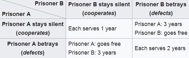
Prisoner’s dilemma graphic. Source: Wikipedia

Binomial probability Binomial means it has one of only two outcomes such as heads or tails. A binomial experiment is one that possesses the following properties:

• The experiment consists of n repeated trials
• Each trial results in an outcome that may be classified as a success or a failure (hence the name, binomial)
• The probability of a success, denoted by p, remains constant from trial to trial and repeated trials are independent.

The number of successes X in n trials of a binomial experiment is called a binomial random variable. The probability distribution of the random variable X is called a binomial distribution.

Type I and type II errors Type I error is where a true hypothesis is rejected. Type II error is where a false hypothesis is accepted.

Confidence interval Used in surveys, the confidence interval is a range of values, above and below a finding, in which the actual value is likely to fall. The confidence interval represents the accuracy or precision of an estimate.

Central limit theorem In probability theory, the central limit theorem (CLT) establishes that, in some situations, when independent random variables are added, their properly normalized sum tends toward a normal distribution (informally a “bell curve”) even if the original variables themselves are not normally distributed. OR: the sum or average of a large bunch of measurements follows a normal curve even if the individual measurements themselves do not. OR: averages and sums of non-normally distributed quantities will nevertheless themselves have a normal distribution. OR:

Under a wide variety of circumstances, averages (or sums) of even non-normally distributed quantities will nevertheless have a normal distribution (p.179)

Regression analysis here are many types of regression analysis, at their core they all examine the influence of one or more independent variables on a dependent variable. Performing a regression allows you to confidently determine which factors matter most, which factors can be ignored, and how these factors influence each other. In order to understand regression analysis you must comprehend the following terms:

• Dependent Variable: This is the factor you’re trying to understand or predict.
• Independent Variables: These are the factors that you hypothesize have an impact on your dependent variable.

Correlation is not causation a principle which cannot be repeated too often.

Gaussian distribution Gaussian distribution (also known as normal distribution) is a bell-shaped curve, and it is assumed that during any measurement values will follow a normal distribution with an equal number of measurements above and below the mean value.

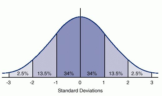
The normal distribution is the most important probability distribution in statistics because it fits so many natural phenomena. For example, heights, blood pressure, measurement error, and IQ scores follow the normal distribution.

Statistical significance A result is statistically significant if it is sufficiently unlikely to have occurred by chance.

2. A Mathematician Reads the Newspaper: Making Sense of the Numbers in the Headlines

Incidence matrices In mathematics, an incidence matrix is a matrix that shows the relationship between two classes of objects. If the first class is X and the second is Y, the matrix has one row for each element of X and one column for each element of Y. The entry in row x and column y is 1 if x and y are related (called incident in this context) and 0 if they are not. Paulos creates an incidence matrix to show

Complexity horizon On the analogy of an ‘event horizon’ in physics, Paulos suggests this as the name for levels of complexity in society around us beyond which mathematics cannot go. Some things just are too complex to be understood using any mathematical tools.

Nonlinear complexity Complex systems often have nonlinear behavior, meaning they may respond in different ways to the same input depending on their state or context. In mathematics and physics, nonlinearity describes systems in which a change in the size of the input does not produce a proportional change in the size of the output.

The Banzhaf power index is a power index defined by the probability of changing an outcome of a vote where voting rights are not necessarily equally divided among the voters or shareholders. To calculate the power of a voter using the Banzhaf index, list all the winning coalitions, then count the critical voters. A critical voter is a voter who, if he changed his vote from yes to no, would cause the measure to fail. A voter’s power is measured as the fraction of all swing votes that he could cast. There are several algorithms for calculating the power index.

Vector field may be thought of as a rule f saying that ‘if an object is currently at a point x, it moves next to point f(x), then to point f(f(x)), and so on. The rule f is non-linear if the variables involved are squared or multiplied together and the sequence of the object’s positions is its trajectory.

Chaos theory (1960) is a branch of mathematics focusing on the behavior of dynamical systems that are highly sensitive to initial conditions.

‘Chaos’ is an interdisciplinary theory stating that within the apparent randomness of chaotic complex systems, there are underlying patterns, constant feedback loops, repetition, self-similarity, fractals, self-organization, and reliance on programming at the initial point known as sensitive dependence on initial conditions.

The butterfly effect describes how a small change in one state of a deterministic nonlinear system can result in large differences in a later state, e.g. a butterfly flapping its wings in Brazil can cause a hurricane in Texas.

Linear models are used more often not because they are more accurate but because that are easier to handle mathematically.

All mathematical systems have limits, and even chaos theory cannot predict even relatively simple nonlinear situations.

Zipf’s Law states that given a large sample of words used, the frequency of any word is inversely proportional to its rank in the frequency table. So word number n has a frequency proportional to 1/n. Thus the most frequent word will occur about twice as often as the second most frequent word, three times as often as the third most frequent word, etc. For example, in one sample of words in the English language, the most frequently occurring word, “the”, accounts for nearly 7% of all the words (69,971 out of slightly over 1 million). True to Zipf’s Law, the second-place word “of” accounts for slightly over 3.5% of words (36,411 occurrences), followed by “and” (28,852). Only about 135 words are needed to account for half the sample of words in a large sample

Benchmark estimates Benchmark numbers are numbers against which other numbers or quantities can be estimated and compared. Benchmark numbers are usually multiples of 10 or 100.

Non standard models Almost everyone, mathematician or not, is comfortable with the standard model (N : +, ·) of arithmetic. Less familiar, even among logicians, are the non-standard models of arithmetic.

The S-curve A sigmoid function is a mathematical function having a characteristic “S”-shaped curve or sigmoid curve. Often, sigmoid function refers to the special case of the logistic function shown below

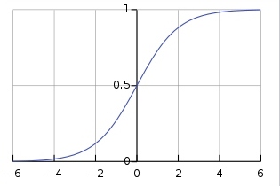
and defined by the formula:

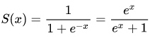
This curve, sometimes called the logistic curve is extremely widespread: it appears to describe the growth of entities as disparate as Mozart’s symphony production, the rise of airline traffic, and the building of Gothic cathedrals (p.91)

Differential calculus The study of rates of change, rates of rates of change, and the relations among them.

Algorithm complexity gives on the length of the shortest program (algorithm) needed to generate a given sequence (p.123)

Chaitin’s theorem states that every computer, every formalisable system, and every human production is limited; there are always sequences that are too complex to be generated, outcomes too complex to be predicted, and events too dense to be compressed (p.124)

Simpson’s paradox (1951) A phenomenon in probability and statistics, in which a trend appears in several different groups of data but disappears or reverses when these groups are combined.

The amplification effect of repeated playing the same game, rolling the same dice, tossing the same coin.

Related links

• A Mathematician Reads the Newspaper: Making Sense of the Numbers in the Headlines on Amazon
• Innumeracy: Mathematical Illiteracy and Its Consequences on Amazon
• John Allen Paulos’s website

Reviews of other science books

Chemistry

• The Periodic Kingdom: A Journey Into the Land of the Chemical Elements by Peter Atkins (1995)

Cosmology

• The Perfect Theory by Pedro G. Ferreira (2014)
• The Book of Universes by John D. Barrow (2011)
• The Origin Of The Universe: To the Edge of Space and Time by John D. Barrow (1994)
• The Last Three Minutes: Conjectures about the Ultimate Fate of the Universe by Paul Davies (1994)
• A Brief History of Time: From the Big Bang to Black Holes by Stephen Hawking (1988)
• The Black Cloud by Fred Hoyle (1957)

The Environment

• The Sixth Extinction: An Unnatural History by Elizabeth Kolbert (2014)
• The Sixth Extinction by Richard Leakey and Roger Lewin (1995)

Genetics and life

• Life At The Speed of Light: From the Double Helix to the Dawn of Digital Life by J. Craig Venter (2013)
• What Is Life? How Chemistry Becomes Biology by Addy Pross (2012)
• Seven Clues to the Origin of Life by A.G. Cairns-Smith (1985)
• The Double Helix by James Watson (1968)

Human evolution

• The Origin of Our Species by Chris Stringer (2011)
• Guns, Germs and Steel by Jared Diamond (1997)

Maths

• Alex’s Adventures in Numberland by Alex Bellos (2010)
• Nature’s Numbers: Discovering Order and Pattern in the Universe by Ian Stewart (1995)
• Innumeracy: Mathematical Illiteracy and Its Consequences by John Allen Paulos (1988)
• A Mathematician Reads the Newspaper: Making Sense of the Numbers in the Headlines by John Allen Paulos (1995)

Particle physics

• Atomic by Jim Baggott (2009)

Psychology

• Tips For Trying To Think Less Irrationally
• Irrationality: The Enemy Within by Stuart Sutherland (1992)
• Judgement Under Uncertainty: Heuristics and Biases by Amos Tversky and Daniel Kahneman (1974)